With the advancement of computer technology, FDTD-Finite Difference TIme Domain can study microwave circuits more and more widely, from passive circuits to active circuits, from linear circuits to nonlinear circuits. From TEM system to dispersion system, FDTD has been successfully applied.
However, when the geometry of the circuit is relatively complicated and the electrical size of the circuit is large, the computer memory used or the calculation time required is very large, and even in some cases, even if the calculation time is consumed, it cannot be obtained. The precision required. For example, in the analysis of the waveguide diaphragm filter, in order to correctly simulate the geometry of all the diaphragms, the grid size of the FDTD grid is chosen to be very small, resulting in a very large number of grids describing the entire waveguide filter. Since there is a uniform waveguide transmission line between every two diaphragms, it is obviously unnecessary to use the same grid as the diaphragm. People have used a non-uniform FDTD grid to solve this problem. When the size of the grid is relatively large, not only is the convergence difficult to control, but it still cannot save computation time. The DiakopTIcs idea is applied to the full-wave analysis of the microwave circuit. By dividing the circuit into several independent parts, different meshes are used according to the specific structure of each part, and the full-wave time-domain analysis is performed on each part independently, due to the The grid is uniform, so it is easy to guarantee the convergence of the algorithm.
Second, the concept of DiakopTIcsDiakopTIcs is defined as: decomposing a circuit into a number of relatively simple sub-circuits, independently calculating the characteristics of the sub-circuits, and coupling the sub-circuits through connection conditions. The characteristics of the sub-circuit in the linear circuit theory are represented by the impulse response function; the coupling between the sub-circuits is accomplished by both serial and parallel algorithms. The serial algorithm connects from either end of the circuit to the other end, and sequentially considers the sub-circuit viewed from the reference plane as the load of the previous sub-circuit, finds the input characteristics of the equivalent sub-circuit, and This input characteristic is regarded as the load of the previous sub-circuit... The serial algorithm is simple and easy to write a computer program, but the problem is: when a sub-circuit in the circuit needs to be adjusted, connect after the sub-circuit The parts must be reconnected, and all connection calculations can only be performed sequentially in time and space, and the computational efficiency is low; the parallel algorithm can start from any position in the circuit and simultaneously calculate the connection of several sub-circuits adjacent to each other. And the adjustment of the characteristics of a certain sub-circuit does not affect the connection of other sub-circuits, especially when the characteristics of a sub-circuit need to be repeatedly adjusted, the connection calculation for the remaining sub-circuits only needs to be performed once.
When studying the microwave circuit problem, if the microwave circuit can be equivalent to a linear network, it can be assumed that the Green's function describing the characteristics of the microwave circuit can correspond to the impulse response function in the circuit theory. From the perspective of electromagnetic field theory, the time domain Green's function g(r, t; r0, t0) is the field of the unit shock signal applied at the point source t0 at the r0 point at the observation point r and t, and satisfies the equation.
![]() (1)
(1)
When two microwave sub-circuits are connected, there is a complex coupling relationship on the connection reference surface. This coupling relationship can be visualized by electromagnetic waves reflected and transmitted in a medium with two discontinuous interfaces, as shown in Fig. 1. . So how do you apply the Diakoptics algorithm to the analysis of microwave circuit characteristics? Before introducing this point, this article first briefly introduces the mathematical description of the Diakoptics algorithm.
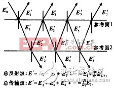
Figure 1 The reflection and transmission phenomena in the medium can be used to graphically describe the coupling relationship between two microwave sub-circuits.
Third, the mathematical description of the Diakoptics algorithmA mathematical description of the Diakoptics algorithm is given in a string, parallel connection of two two-port networks. Figure 2 assumes that the impulse response functions of the reflected and transmitted waves of the two sub-circuits are: gr1(t), gr2(t), gt1(t), gt2(t) and hr1(t), hr2(t), ht1( t), ht2(t), the superscript "r" denotes a reflected wave, "t" denotes a transmitted wave, the subscript 1 denotes an excitation from the input reference facing circuit, and the subscript 2 denotes an excitation from the output reference facing the circuit. Let f be the impulse response function of the circuit after the two sub-circuits are connected. Using the serial algorithm, the impulse response seen from the f network input reference plane is:
Fr1(t)=gr1(t)+gt2(t)*hr1(t)*gt1(t)+gt2(t)*hr1(t)
*gr2(t)*hr1(t)*gt1(t)+...+gt2(t)*(hr1(t)
*gr2(t))n*hr1(t)*gt1(t)+...; (2)
Using the parallel algorithm, the impulse response functions fr1(t), ft2(t) seen from the input port of the f-circuit and the impulse response function fr2(t), ft1(t) seen from the output port of the f-circuit are:
Fr1(t)=gr1(t)+gt2(t)*hr1(t)*gt1(t)+gt2(t)*hr1(t)
*gr2(t)*hr1(t)*gt1(t)+...+gt2(t)*(hr1(t)
*gr2(t))n*hr1(t)*gt1(t)+...
Ft2(t)=gt2(t)*hr2(t)+gt2(t)*hr1(t)*gr2(t)*ht2(t)+...
+gr2(t)*(hr1(t)*gr2(t))n*hr2(t)+... (3)
Fr2(t)=hr2(t)+ht1(t)*gr2(t)*ht2(t)+ht1(t)*gr2(t)
*hr1(t)*gt2(t)*ht2(t)+...+ht1(t)*(gr2(t)
*hr1(t))n*gr2(t)*ht2(t)+...
Ft1(t)=ht1(t)*gt1(t)+ht1(t)*gr2(t)*hr1(t)*gt1(t)+...
+ht1(t)*(gr2(t)*hr1(t))n*gr1(t)+...
Among them, * represents the time domain convolution, and the meaning of the superscript is unchanged.

Figure 2 illustrates the two subcircuit connections of the Diakoptics algorithm.
When the multi-port sub-circuit is connected, the above algorithm is still valid, except that each impact function in the formula should be changed to the corresponding sub-matrix. For example, let g network be M+N port network with M ports at the input end and N ports at the output end, h network is N+L port network with N ports at the input end and L ports at the output end (g and h phase The number of adjacent ports should be the same.) The reflection and transmission sub-matrices at the g network input reference plane are:
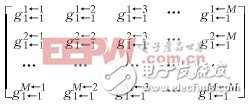
with
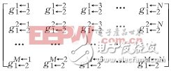
The subscript in the formula represents the reference plane, iâ†j means: i is the reference plane of the response, j is the reference plane of the excitation; the superscript represents the port, mâ†n means: n is the input port, m is the output port . Similarly, the reflection and transmission sub-matrices at the g network output reference plane are:
with

The corresponding submatrices of the h network can be obtained in the same way. The impact response function [f] of the connected network is:
[fr1(t)]=[gr1(t)]+[gt2(t)]*[hr1(t)]*[gt1(t)]+[gt2(t)]
*[hr1(t)]*[gr2(t)]*[hr1(t)]*[gt1(t)]+...
[ft2(t)]=[gt2(t)]*[ht2(t)]+[gt2(t)]*[hr1(t)]*[gr2(t)]*[ht2(t)]+...
[fr2(t)]=[hr2(t)]+[ht1(t)]*[gr2(t)]*[ht2(t)]+[ht1(t)]
*[gr2(t)]*[hr1(t)]*[gr2(t)]*[ht2(t)]+...
[ft1(t)]=[ht1(t)]*[gt1(t)]+[ht1(t)]*[gr2(t)]*[hr1(t)]*[gt1(t)]+... (4)
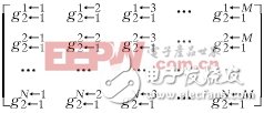
Where [fr1(t)], [ft1(t)], [fr2(t)], and [ft2(t)] are M×M, L×M, L×L, and M×L order sub-matrices, respectively. Let's take [gt2(t)]*[ht2(t)] as an example to illustrate how to calculate the matrix convolution, and take the first element of [gt2(t)]*[ht2(t)] as an example to illustrate its physics. significance:
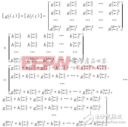 (5)
(5)
G1â†11â†2*h1â†11â†2:h The output of the first port on the sub-network output reference plane is output through the first port of the gh connection plane on the input interface of the g sub-network input reference plane; g1 â†21â†2*h2â†11â†2:h The output of the first port on the sub-network output reference plane is output through the second port of the gh interface on the input interface of the g sub-network input reference plane; g1↠N1â†2*hNâ†11â†2:h The input of the first port on the sub-network output reference plane is coupled through the Nth port of the gh interface, and the output generated by port 1 on the g sub-network input reference plane; therefore [ The first element of gt2(t)]*[ht2(t)] describes the output of the first port on the h network output reference plane coupled to the first port of the g network input reference plane.
Implementation of Diakoptics Algorithm in Microwave Circuit AnalysisDiakoptics is derived from network theory. In order to apply it to the analysis of microwave circuits, it is first necessary to establish an equivalent circuit model for microwave circuits suitable for using the Diakoptics method.
1. Equivalent time domain network model of microwave circuit
The basic method for establishing the equivalent time domain network model of microwave circuits is to use the basis function technique (or time domain mode technique) to represent the field at the reference plane as a linear combination of selected orthogonal basis functions, a microwave network, etc. It is a multi-mode circuit, and then the multi-mode circuit is equivalent to a multi-port network.
The selected basis function satisfies the following conditions: only a function of spatial coordinates; independent of time; constitutes a complete orthogonal set. And for a given microwave circuit, the selected basis function should be able to effectively describe the distribution of electromagnetic fields in the circuit. Assume that the XY plane is the plane of the circuit cross section and Z is the propagation direction. The electric field distribution of the circuit at z=z0 under the Dirac-δ function excitation is Ei(x, y, z0, t), {φmn(x, y )} is a family of basis functions, using φmm(x, y) to represent the field at t=t0,z=z0 in the microwave circuit as:
![]() (6)
(6)
Where amn(z0, t0) is the coefficient of the (m, n)th basis function, ie the amplitude, so that the microwave circuit seen from the reference plane z=z0 can be equivalent to an equivalent time domain multimode based on the basis function. Circuit. The functional form of the basis function can be either an orthogonal function form suitable for a general circuit or a special orthogonal function particularly suitable for a certain type of circuit. Generally speaking, when the circuit geometry is relatively complicated and it is not easy to select a special orthogonal function as a basis function according to the circuit characteristics, a rectangular pulse function can be selected (taking the value of the mesh node as the average value of the entire mesh, so the pulse width For the width of a grid). However, the pulse function describes only the local information of the system, so to achieve sufficient precision, the function has more expansion items. When the orthogonal function can effectively represent the global information of the circuit, usually only a few or a dozen items are needed to achieve the required precision. For example, for a uniformly filled rectangular waveguide problem, such as selecting a {sin, cos} orthogonal function set based on the distribution characteristics of the field within the waveguide, usually only five items are required. In comparison, at least 60 pulses, or 60 nodes, are needed to more accurately describe the spatial field distribution on the cross section of the waveguide system.
The orthogonality of the basis functions allows each basis function to be treated as a separate port, so the above-described basis-based equivalent time domain multimode circuit can be further considered as a multi-port network.
2. Calculation of equivalent multi-port network characteristics
The spectrum of the impact function is infinitely wide, so the impact response function of the system cannot be directly solved by FDTD algorithm. FDTD-Diakoptics uses Gaussian pulse modulated wave as excitation, and the impact response function of finite bandwidth microwave circuit is obtained by windowed Fourier transform technique. . The modulation frequency of the Gaussian pulse excitation is the center frequency of the operating band of the circuit, and the sampling interval of the pulse width and the pulse time depends on the frequency resolution and the bandwidth. Although the excitation pulse has a finite bandwidth, the impact response function obtained by FDTD-Diakoptics includes the effect of windowing (referred to as the quasi-impact response function at this time), but as long as the following conditions are met: FDTD- When Diakoptics analyzes the entire circuit characteristics, each sub-circuit uses an excitation pulse with the same spectral characteristics to account for the broadening effect of windowing on the time domain pulse, and the resulting frequency response of the impulse response function is sufficiently accurate.
V. FDTD-Diakoptics application examples and discussion In this paper, the application of a waveguide bandpass filter is taken as an example to illustrate the application of the algorithm. Figure 3 shows a rectangular waveguide bandpass filter (WR34) with five diaphragms. According to the method, the filter is first divided into five parts, which are calculated by FDTD, and the field distribution at all connected reference planes (shown by the dotted line in the figure) is obtained. In the FDTD calculation, the Gaussian pulse modulation function is: f(t)=AmaxA(x,y)exp[-((t-t0)/T)2].sin(2πf0t), where the modulation frequency f0 is the center frequency of the WR34-TE10 mode single mode operating band; A( x, y) is the spatial distribution of the excitation amplitude. The Diakoptics algorithm needs to calculate the response of all possible base functions with a single excitation, so A(x, y) is selected as each basis function. The amplitude Amax of the excitation function depends on its attenuation along the propagation direction and the accuracy of calculation. The basic principle is that the field at the discontinuity and the observation surface still has a large enough amplitude. The value of T must be guaranteed to be cut off on the spectrum of the excitation pulse. The energy at the frequency point has a sufficiently small value. In this example, the single-mode operating band of WR34 is: fTE10=17.369 GHz, fTE20=34.738 GHz, f0=26.0535 GHz, T=200 (ps), t0=3T, Amax=10, and the basis function is φn(x)= Sin ![]() The corresponding coefficient an(z0,t) is shown in Figure 4 (only one result is given due to the length of the article). Figure 5 shows the filter frequency characteristics obtained by the method of this paper. It can be seen that the results agree well with the FDTD results.
The corresponding coefficient an(z0,t) is shown in Figure 4 (only one result is given due to the length of the article). Figure 5 shows the filter frequency characteristics obtained by the method of this paper. It can be seen that the results agree well with the FDTD results.
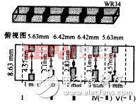
Figure 3 Schematic diagram of five diaphragm WR34 waveguide bandpass filter
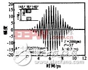
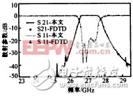
Fig. 4 The coefficient of the reflected wave basis function of the first sub-circuit in Fig. 3 obtained by the method in this paperFig. 5 The frequency characteristics of the WR34 waveguide filter shown in Fig. 3.
ConclusionThis paper introduces a new method for analyzing complex microwave circuits: FDTD-Diakoptics method, which can overcome the shortcomings of traditional FDTD methods requiring large memory and long calculation time, and can fully exploit the advantages of FDTD to easily study complex geometric circuits. Some examples of the author's analysis and design prove that this method is not only flexible, but also has high precision. It is a relatively effective microwave circuit simulation analysis method.
Floor-Standing Advertising Display
Floor Standing Lcd Advertising Display,Vertical Advertising Display,Vertical Advertising Lcd Display,Vertical Advertising Screen
Guangdong Elieken Electronic Technology Co.,Ltd. , https://www.elieken.com